
In this case study, we review an implementation of the Multivariate Singualr Spectrum Analysis (mSSA) algorithm developed by MIT professors Anish Agarwal, Abdullah Alomar, and Devavrat Shah. We will be using the Electricity Load dataset from UCI Machine Learning Repository. The dataset describes the 15-minutes load for 370 different clients in kW. Each column represents one client. The dataset has electricity consumption for these 370 houses every 15 mins starting from 2011-01-01, till 2015-01-01. Some clients are created after 2011. In these cases, consumption was considered zero.
Build a forecasting model to forecast the electricity load of different clients (i.e., forecasting multiple time series at once) for a certain period in the future.
This algorithm is known as Multivariate Singular Spectrum Analysis (mSSA). This matrix factorization method is useful for:
To learn more about this algorithm, please refer to this paper
The python library to use this algorithm is not currently present in PyPi. The code repository is present in this GitHub repository: https://github.com/AbdullahO/mSSA. So we will be using a different way to install the library on your local machine. Below we have provided the steps to follow to install this library.
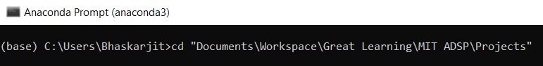
git clone https://github.com/AbdullahO/mSSA.git as shown below: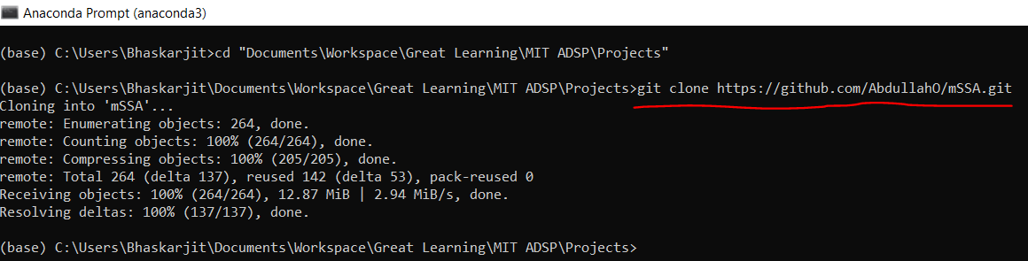
mSSA in the directory where you have cloned the repository as shown below:
cd mSSA, as shown below: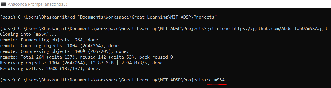
pip3 install ., as shown below: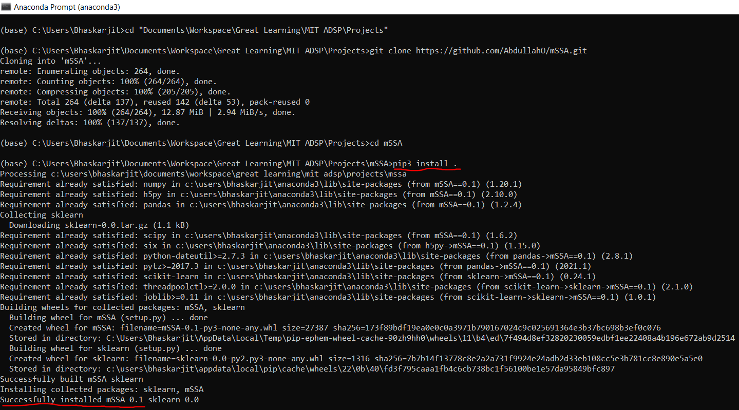
Now, the library is installed, and you are ready to use this for time series forecasting.
import io

# Python packages for numerical and data frame operations
import numpy as np
import pandas as pd

# Installing the mSSA library
from mssa.mssa import mSSA

# An advanced library for data visualization in python
import seaborn as sns

# A simple library for data visualization in python
import matplotlib.pyplot as plt

# To ignore warnings in the code
import warnings
warnings.filterwarnings('ignore')
The dataset is in a zipped file we will use the below piece of code to unzip the file
import requests
import zipfile
import io

# Download the file
url = "https://archive.ics.uci.edu/ml/machine-learning-databases/00321/LD2011_2014.txt.zip"
response = requests.get(url)
zip_file = zipfile.ZipFile(io.BytesIO(response.content))

# Extract the contents
zip_file.extractall()

# Perform text manipulation
with open("LD2011_2014.txt", "r") as file:
    content = file.read()

content = content.replace(",", ".")  # Replace commas with dots

with open("LD2011_2014_clean.txt", "w") as file:
    file.write(content)
Once unzip is complete, go to your working directory, you will find a text file named LD2011_2014.txt. And check the data by opening this file you will see all the values are separated by ;. Now we will load this dataset in this notebook session.
# Reading the dataset
data = pd.read_csv('LD2011_2014.txt', sep = ';')

# Let us see the first five records of the dataset
data.head()
| Unnamed: 0 | MT_001 | MT_002 | MT_003 | MT_004 | MT_005 | MT_006 | MT_007 | MT_008 | MT_009 | ... | MT_361 | MT_362 | MT_363 | MT_364 | MT_365 | MT_366 | MT_367 | MT_368 | MT_369 | MT_370 | |
|---|---|---|---|---|---|---|---|---|---|---|---|---|---|---|---|---|---|---|---|---|---|
| 0 | 2011-01-01 00:15:00 | 0 | 0 | 0 | 0 | 0 | 0 | 0 | 0 | 0 | ... | 0 | 0.0 | 0 | 0 | 0 | 0 | 0 | 0 | 0 | 0 |
| 1 | 2011-01-01 00:30:00 | 0 | 0 | 0 | 0 | 0 | 0 | 0 | 0 | 0 | ... | 0 | 0.0 | 0 | 0 | 0 | 0 | 0 | 0 | 0 | 0 |
| 2 | 2011-01-01 00:45:00 | 0 | 0 | 0 | 0 | 0 | 0 | 0 | 0 | 0 | ... | 0 | 0.0 | 0 | 0 | 0 | 0 | 0 | 0 | 0 | 0 |
| 3 | 2011-01-01 01:00:00 | 0 | 0 | 0 | 0 | 0 | 0 | 0 | 0 | 0 | ... | 0 | 0.0 | 0 | 0 | 0 | 0 | 0 | 0 | 0 | 0 |
| 4 | 2011-01-01 01:15:00 | 0 | 0 | 0 | 0 | 0 | 0 | 0 | 0 | 0 | ... | 0 | 0.0 | 0 | 0 | 0 | 0 | 0 | 0 | 0 | 0 |
5 rows × 371 columns
As you can see above, the first column name is blank, and this is the time of the dataset as this is a time-series dataset.
# Let us see the bottom five records of the dataset
data.tail()
| Unnamed: 0 | MT_001 | MT_002 | MT_003 | MT_004 | MT_005 | MT_006 | MT_007 | MT_008 | MT_009 | ... | MT_361 | MT_362 | MT_363 | MT_364 | MT_365 | MT_366 | MT_367 | MT_368 | MT_369 | MT_370 | |
|---|---|---|---|---|---|---|---|---|---|---|---|---|---|---|---|---|---|---|---|---|---|
| 140251 | 2014-12-31 23:00:00 | 2,53807106598985 | 22,0483641536273 | 1,73761946133797 | 150,406504065041 | 85,3658536585366 | 303,571428571429 | 11,3058224985868 | 282,828282828283 | 68,1818181818182 | ... | 276,945039257673 | 28200.0 | 1616,03375527426 | 1363,63636363636 | 29,986962190352 | 5,85137507314219 | 697,102721685689 | 176,961602671119 | 651,026392961877 | 7621,62162162162 |
| 140252 | 2014-12-31 23:15:00 | 2,53807106598985 | 21,3371266002845 | 1,73761946133797 | 166,666666666667 | 81,7073170731707 | 324,404761904762 | 11,3058224985868 | 252,525252525253 | 64,6853146853147 | ... | 279,800142755175 | 28300.0 | 1569,62025316456 | 1340,90909090909 | 29,986962190352 | 9,94733762434172 | 671,641791044776 | 168,614357262104 | 669,354838709677 | 6702,7027027027 |
| 140253 | 2014-12-31 23:30:00 | 2,53807106598985 | 20,6258890469417 | 1,73761946133797 | 162,60162601626 | 82,9268292682927 | 318,452380952381 | 10,1752402487281 | 242,424242424242 | 61,1888111888112 | ... | 284,796573875803 | 27800.0 | 1556,96202531646 | 1318,18181818182 | 27,3794002607562 | 9,3622001170275 | 670,763827919227 | 153,589315525876 | 670,087976539589 | 6864,86486486487 |
| 140254 | 2014-12-31 23:45:00 | 1,26903553299492 | 21,3371266002845 | 1,73761946133797 | 166,666666666667 | 85,3658536585366 | 285,714285714286 | 10,1752402487281 | 225,589225589226 | 64,6853146853147 | ... | 246,252676659529 | 28000.0 | 1443,03797468354 | 909,090909090909 | 26,0756192959583 | 4,09596255119953 | 664,618086040386 | 146,911519198664 | 646,627565982405 | 6540,54054054054 |
| 140255 | 2015-01-01 00:00:00 | 2,53807106598985 | 19,9146514935989 | 1,73761946133797 | 178,861788617886 | 84,1463414634146 | 279,761904761905 | 10,1752402487281 | 249,158249158249 | 62,9370629370629 | ... | 188,436830835118 | 27800.0 | 1409,28270042194 | 954,545454545455 | 27,3794002607562 | 4,09596255119953 | 628,621597892889 | 131,886477462437 | 673,020527859238 | 7135,13513513513 |
5 rows × 371 columns
And also, if you look above, the fractional part of the numbers are separated by , instead of .. We need to fix this as well. There are many different ways of doing this data cleaning. But here, we will fix these issues while loading the dataset itself. So we need to delete the existing data frame and load it differently so that we can fix the issues mentioned.
# Removing the existing data frame
del data
# Loading the data again
data = pd.read_csv('LD2011_2014.txt', sep = ';', decimal = ',')
# See the first five records of the dataset.
data.head()
| Unnamed: 0 | MT_001 | MT_002 | MT_003 | MT_004 | MT_005 | MT_006 | MT_007 | MT_008 | MT_009 | ... | MT_361 | MT_362 | MT_363 | MT_364 | MT_365 | MT_366 | MT_367 | MT_368 | MT_369 | MT_370 | |
|---|---|---|---|---|---|---|---|---|---|---|---|---|---|---|---|---|---|---|---|---|---|
| 0 | 2011-01-01 00:15:00 | 0.0 | 0.0 | 0.0 | 0.0 | 0.0 | 0.0 | 0.0 | 0.0 | 0.0 | ... | 0.0 | 0.0 | 0.0 | 0.0 | 0.0 | 0.0 | 0.0 | 0.0 | 0.0 | 0.0 |
| 1 | 2011-01-01 00:30:00 | 0.0 | 0.0 | 0.0 | 0.0 | 0.0 | 0.0 | 0.0 | 0.0 | 0.0 | ... | 0.0 | 0.0 | 0.0 | 0.0 | 0.0 | 0.0 | 0.0 | 0.0 | 0.0 | 0.0 |
| 2 | 2011-01-01 00:45:00 | 0.0 | 0.0 | 0.0 | 0.0 | 0.0 | 0.0 | 0.0 | 0.0 | 0.0 | ... | 0.0 | 0.0 | 0.0 | 0.0 | 0.0 | 0.0 | 0.0 | 0.0 | 0.0 | 0.0 |
| 3 | 2011-01-01 01:00:00 | 0.0 | 0.0 | 0.0 | 0.0 | 0.0 | 0.0 | 0.0 | 0.0 | 0.0 | ... | 0.0 | 0.0 | 0.0 | 0.0 | 0.0 | 0.0 | 0.0 | 0.0 | 0.0 | 0.0 |
| 4 | 2011-01-01 01:15:00 | 0.0 | 0.0 | 0.0 | 0.0 | 0.0 | 0.0 | 0.0 | 0.0 | 0.0 | ... | 0.0 | 0.0 | 0.0 | 0.0 | 0.0 | 0.0 | 0.0 | 0.0 | 0.0 | 0.0 |
5 rows × 371 columns
# See the bottom five records of the dataset
data.tail()
| Unnamed: 0 | MT_001 | MT_002 | MT_003 | MT_004 | MT_005 | MT_006 | MT_007 | MT_008 | MT_009 | ... | MT_361 | MT_362 | MT_363 | MT_364 | MT_365 | MT_366 | MT_367 | MT_368 | MT_369 | MT_370 | |
|---|---|---|---|---|---|---|---|---|---|---|---|---|---|---|---|---|---|---|---|---|---|
| 140251 | 2014-12-31 23:00:00 | 2.538071 | 22.048364 | 1.737619 | 150.406504 | 85.365854 | 303.571429 | 11.305822 | 282.828283 | 68.181818 | ... | 276.945039 | 28200.0 | 1616.033755 | 1363.636364 | 29.986962 | 5.851375 | 697.102722 | 176.961603 | 651.026393 | 7621.621622 |
| 140252 | 2014-12-31 23:15:00 | 2.538071 | 21.337127 | 1.737619 | 166.666667 | 81.707317 | 324.404762 | 11.305822 | 252.525253 | 64.685315 | ... | 279.800143 | 28300.0 | 1569.620253 | 1340.909091 | 29.986962 | 9.947338 | 671.641791 | 168.614357 | 669.354839 | 6702.702703 |
| 140253 | 2014-12-31 23:30:00 | 2.538071 | 20.625889 | 1.737619 | 162.601626 | 82.926829 | 318.452381 | 10.175240 | 242.424242 | 61.188811 | ... | 284.796574 | 27800.0 | 1556.962025 | 1318.181818 | 27.379400 | 9.362200 | 670.763828 | 153.589316 | 670.087977 | 6864.864865 |
| 140254 | 2014-12-31 23:45:00 | 1.269036 | 21.337127 | 1.737619 | 166.666667 | 85.365854 | 285.714286 | 10.175240 | 225.589226 | 64.685315 | ... | 246.252677 | 28000.0 | 1443.037975 | 909.090909 | 26.075619 | 4.095963 | 664.618086 | 146.911519 | 646.627566 | 6540.540541 |
| 140255 | 2015-01-01 00:00:00 | 2.538071 | 19.914651 | 1.737619 | 178.861789 | 84.146341 | 279.761905 | 10.175240 | 249.158249 | 62.937063 | ... | 188.436831 | 27800.0 | 1409.282700 | 954.545455 | 27.379400 | 4.095963 | 628.621598 | 131.886477 | 673.020528 | 7135.135135 |
5 rows × 371 columns
Now, you can see that the issues are fixed.
Next, we will pre-process the dataset further. Specifically, we will:
# Removing data before 2012
data = data.iloc[8760 * 4:]

# Picking the first 20 houses and saving it to another variable data_small
data_small = data.iloc[ :, : 21]

# Aggregating the data
data_small['time'] = pd.to_datetime(data_small['Unnamed: 0']).dt.ceil('1h')

data_small = data_small.drop(['Unnamed: 0'], axis = 1)

agg_dict = {}
for col in data_small.columns[ :-1]:
    agg_dict[col] = 'mean'

final_data = data_small.groupby(['time']).agg(agg_dict)
print('data aggregated..')

# See the shape of the data
data_small.shape
data aggregated..
(105216, 21)
# Let us see the first five records in the final_data
final_data.head()
| MT_001 | MT_002 | MT_003 | MT_004 | MT_005 | MT_006 | MT_007 | MT_008 | MT_009 | MT_010 | MT_011 | MT_012 | MT_013 | MT_014 | MT_015 | MT_016 | MT_017 | MT_018 | MT_019 | MT_020 | |
|---|---|---|---|---|---|---|---|---|---|---|---|---|---|---|---|---|---|---|---|---|
| time | ||||||||||||||||||||
| 2012-01-01 01:00:00 | 4.124365 | 22.759602 | 77.324066 | 138.211382 | 72.256098 | 348.214286 | 8.620690 | 279.461279 | 72.989510 | 87.903226 | 59.798808 | 0.0 | 47.678275 | 36.534780 | 0.0 | 55.096811 | 76.145553 | 328.274760 | 15.577889 | 55.066079 |
| 2012-01-01 02:00:00 | 4.758883 | 23.115220 | 77.324066 | 137.195122 | 70.121951 | 339.285714 | 6.924816 | 276.094276 | 67.307692 | 82.258065 | 55.886736 | 0.0 | 46.019900 | 34.141672 | 0.0 | 52.249431 | 73.225517 | 305.910543 | 15.452261 | 51.101322 |
| 2012-01-01 03:00:00 | 4.124365 | 22.937411 | 77.324066 | 136.686992 | 66.463415 | 286.458333 | 6.642171 | 239.898990 | 63.811189 | 72.043011 | 54.582712 | 0.0 | 43.532338 | 33.024888 | 0.0 | 43.422551 | 61.994609 | 276.357827 | 14.070352 | 48.458150 |
| 2012-01-01 04:00:00 | 4.758883 | 22.048364 | 77.324066 | 102.134146 | 50.304878 | 191.964286 | 4.804975 | 200.336700 | 41.520979 | 46.236559 | 38.189270 | 0.0 | 35.862355 | 26.005105 | 0.0 | 35.449886 | 46.495957 | 188.498403 | 7.663317 | 39.427313 |
| 2012-01-01 05:00:00 | 4.441624 | 21.870555 | 77.324066 | 81.808943 | 45.121951 | 155.505952 | 3.533070 | 180.134680 | 45.891608 | 42.473118 | 33.904620 | 0.0 | 42.288557 | 24.409700 | 0.0 | 33.599089 | 35.265049 | 160.543131 | 6.155779 | 34.361233 |
As you can see above, each column of the data frame final_data contains hourly reading starting from 2012-01-01 01:00 until 2015-01-01 01:00. Now we will split the observations into training and testing sets. Specifically, the training set will start on at 2012-01-01 01:00 until 2014-12-18 00:00, and the test set will have the rest of the observations.
# Creating training and the testing set
train_data = final_data.loc['2012-12-31' : '2014-12-18']

test_data = final_data.loc['2014-12-19': ]
Let's check how the training and test data looks like
# First five records of the train data
train_data.head()
| MT_001 | MT_002 | MT_003 | MT_004 | MT_005 | MT_006 | MT_007 | MT_008 | MT_009 | MT_010 | MT_011 | MT_012 | MT_013 | MT_014 | MT_015 | MT_016 | MT_017 | MT_018 | MT_019 | MT_020 | |
|---|---|---|---|---|---|---|---|---|---|---|---|---|---|---|---|---|---|---|---|---|
| time | ||||||||||||||||||||
| 2012-12-31 00:00:00 | 2.220812 | 24.182077 | 3.475239 | 151.930894 | 59.451220 | 258.184524 | 6.076880 | 269.360269 | 57.692308 | 62.096774 | 61.289121 | 0.0 | 40.630182 | 35.258456 | 0.0 | 50.825740 | 56.603774 | 245.207668 | 9.673367 | 42.511013 |
| 2012-12-31 01:00:00 | 1.903553 | 23.115220 | 3.475239 | 126.524390 | 54.573171 | 220.982143 | 4.239683 | 245.791246 | 48.513986 | 57.795699 | 46.758569 | 0.0 | 40.630182 | 34.779834 | 0.0 | 41.998861 | 48.068284 | 188.498403 | 7.537688 | 42.951542 |
| 2012-12-31 02:00:00 | 1.586294 | 23.293030 | 3.475239 | 100.101626 | 43.597561 | 186.755952 | 4.098361 | 219.696970 | 42.395105 | 50.806452 | 45.268256 | 0.0 | 42.910448 | 30.631780 | 0.0 | 33.599089 | 43.126685 | 168.530351 | 6.407035 | 33.920705 |
| 2012-12-31 03:00:00 | 1.903553 | 22.403983 | 3.475239 | 89.939024 | 42.682927 | 156.250000 | 3.533070 | 204.545455 | 39.335664 | 48.387097 | 38.561848 | 0.0 | 41.873964 | 28.876835 | 0.0 | 28.473804 | 39.757412 | 155.750799 | 6.407035 | 30.616740 |
| 2012-12-31 04:00:00 | 2.220812 | 22.226174 | 3.475239 | 75.711382 | 38.719512 | 139.880952 | 3.391747 | 230.639731 | 36.276224 | 46.774194 | 31.669151 | 0.0 | 44.776119 | 26.164646 | 0.0 | 28.046697 | 36.837376 | 144.568690 | 5.276382 | 29.074890 |
# First five records of the test set data
test_data.head()
| MT_001 | MT_002 | MT_003 | MT_004 | MT_005 | MT_006 | MT_007 | MT_008 | MT_009 | MT_010 | MT_011 | MT_012 | MT_013 | MT_014 | MT_015 | MT_016 | MT_017 | MT_018 | MT_019 | MT_020 | |
|---|---|---|---|---|---|---|---|---|---|---|---|---|---|---|---|---|---|---|---|---|
| time | ||||||||||||||||||||
| 2014-12-19 00:00:00 | 2.855330 | 20.448080 | 1.737619 | 164.634146 | 92.378049 | 276.785714 | 7.066139 | 274.410774 | 61.625874 | 61.290323 | 47.876304 | 145.744681 | 38.349917 | 54.881940 | 52.944215 | 49.829157 | 51.437556 | 300.319489 | 9.547739 | 47.136564 |
| 2014-12-19 01:00:00 | 2.538071 | 18.669986 | 1.737619 | 136.686992 | 82.621951 | 228.422619 | 4.663652 | 218.855219 | 52.447552 | 49.193548 | 40.983607 | 125.531915 | 39.593698 | 48.181238 | 41.967975 | 38.154897 | 41.554358 | 253.993610 | 9.045226 | 38.546256 |
| 2014-12-19 02:00:00 | 3.172589 | 17.247511 | 1.737619 | 117.378049 | 67.073171 | 198.660714 | 3.815715 | 201.178451 | 44.143357 | 43.817204 | 37.257824 | 118.617021 | 33.996683 | 40.682833 | 37.190083 | 33.314351 | 36.612758 | 230.031949 | 7.914573 | 37.004405 |
| 2014-12-19 03:00:00 | 2.855330 | 16.536273 | 1.737619 | 104.674797 | 60.670732 | 176.339286 | 3.533070 | 175.925926 | 43.269231 | 43.817204 | 34.649776 | 126.063830 | 35.240464 | 39.246969 | 38.094008 | 32.175399 | 34.141959 | 195.686901 | 7.286432 | 33.259912 |
| 2014-12-19 04:00:00 | 2.538071 | 16.358464 | 1.737619 | 105.691057 | 65.243902 | 164.434524 | 3.674392 | 206.228956 | 41.083916 | 47.580645 | 33.718331 | 120.212766 | 39.179104 | 39.566050 | 36.931818 | 29.043280 | 34.141959 | 190.894569 | 7.286432 | 28.634361 |
Let's try to understand how this algorithm works, below is a schematic of this algorithm:
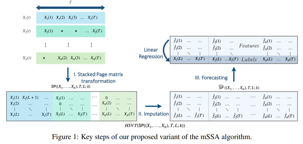
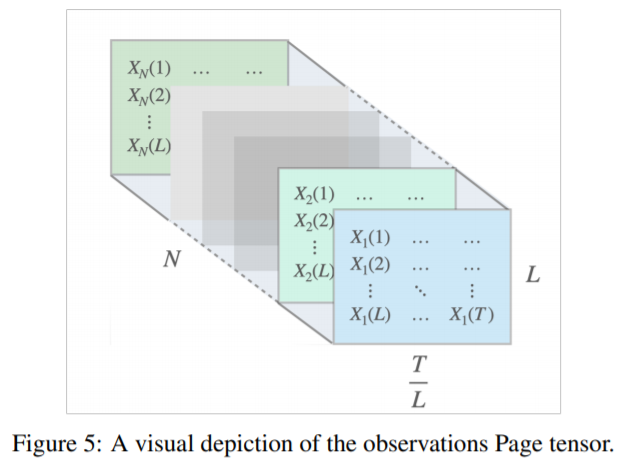
\We can further explore the page matrix as:
As our data is now ready, we can use the algorithm to fit the training data for forecasting. Before fitting the data, let's check what are the hyper-parameters this algorithm uses and what is their meaning?
# To get the details of the algorithm
help(mSSA)
Help on class mSSA in module mssa.mssa:

class mSSA(builtins.object)
 |  mSSA(rank=None, rank_var=1, T=25000000, T_var=None, gamma=0.2, T0=10, col_to_row_ratio=5, agg_method='average', uncertainty_quantification=True, p=None, direct_var=True, L=None, persist_L=None, normalize=True, fill_in_missing=False, segment=False, agg_interval=None, threshold=None)
 |
 |  :param rank: (int) the number of singular values to retain in the means prediction model
 |  :param rank_var: (int) the number of singular values to retain in the variance prediction model
 |  :param gamma: (float) (0,1) fraction of T after which the last sub-model is fully updated
 |  :param segment: (bool) If True, several sub-models will be built, each with a moving windows of length T.
 |  :param T: (int) Number of entries in each submodel in the means prediction model
 |  :param T0: (int) Minimum number of observations to fit a model. (Default 100)
 |  :param col_to_row_ratio: (int) the ratio of no. columns to the number of rows in each sub-model
 |  :param agg_interval: (float) set the interval for pre-processing aggregation step in seconds (if index is timestamps)
 |   or units (if index is integers). Default is None, where the interval will be determined by the median difference
 |   between timestamps.
 |  :param agg_method: Choose one of {'max', 'min', 'average'}.
 |  :param uncertainty_quantification: (bool) if true, estimate the time-varying variance.
 |  :param p: (float) (0,1) select the probability of observation. If None, it will be computed from the observations.
 |  :param direct_var: (bool) if True, calculate variance by subtracting the mean from the observations in the variance
 |  prediction model (recommended), otherwise, the variance model will be built on the squared observations
 |  :param L:  (int) the number of rows in each sub-model. if set, col_to_row_ratio is ignored.
 |  :param normalize: (bool) Normalize the multiple time series before fitting the model.
 |  :param fill_in_missing: if true, missing values will be filled by carrying the last observations forward, and then
 |   carrying the latest observation backward.
 |
 |  Methods defined here:
 |
 |  __init__(self, rank=None, rank_var=1, T=25000000, T_var=None, gamma=0.2, T0=10, col_to_row_ratio=5, agg_method='average', uncertainty_quantification=True, p=None, direct_var=True, L=None, persist_L=None, normalize=True, fill_in_missing=False, segment=False, agg_interval=None, threshold=None)
 |      Initialize self.  See help(type(self)) for accurate signature.
 |
 |  predict(self, col_name, t1, t2=None, num_models=10, confidence_interval=True, use_imputed=False, return_variance=False, confidence=95, uq_method='Gaussian')
 |      Predict 'col_name' at time t1 to time t2.
 |      :param col_name: name of the column to be predicted. It must one of the columns in the original  DF used for
 |      training.
 |      :param t1: (int, or valid timestamp) The initial timestamp to be predicted
 |      :param t2: (int, or valid timestamp) The last timestamp to be predicted, (Optional, Default = t1)
 |      :param num_models: (int, >0) Number of submodels used to create a forecast (Optional, Default = 10)
 |      :param confidence_interval: (bool)  If true, return the (confidence%) confidence interval along with the prediction (Optional, Default = True)
 |      :param confidence: (float, (0,100)) The confidence used to produce the upper and lower bounds
 |      :param use_imputed: (bool)  If true, use imputed values to forecast  (Optional, Default = False)
 |      :param return_variance: (bool)  If true, return mean and variance  (Optional, Default = False, overrides confidence_interval)
 |      :param uq_method: (string): Choose from  {"Gaussian" ,"Chebyshev"}
 |      :return:
 |          DataFrame with the timestamp and predictions
 |
 |  update_model(self, df)
 |      This function takes a new set of entries in a dataframe and update the model accordingly.
 |      if self.segment is set to True, the new entries might build several sub-models  depending on the parameters T and gamma.
 |      :param df: dataframe of new entries to be included in the new model
 |
 |  ----------------------------------------------------------------------
 |  Data descriptors defined here:
 |
 |  __dict__
 |      dictionary for instance variables (if defined)
 |
 |  __weakref__
 |      list of weak references to the object (if defined)
As you can see from above, mSSA class can take several parameters that might affect its performance. Specifically, the parameter rank (int), which determines the number of singular values to retain in the means prediction model. The default value is None, where the model will choose an appropriate rank using the method in the paper:
The Optimal Hard Threshold for Singular Values is 4/√3
We can also tune the 'rank' hyperparameter and choose the optimal value depending on the dataset. Here, we will use rank = 20.
# Let us define the model variable
model = mSSA(rank = 20)

# Updating the model
model.update_model(train_data)
Let's start by forecasting the first day for client MT_020 and comparing it visually with the test data. Now we will produce the forecast for the next day using predict for the range 2014-12-19 01:00:00 to 2014-12-20 00:00:00 along with the 95% confidence interval.
# Define the prediction dataframe
df = model.predict('MT_020', '2014-12-19 01:00:00', '2014-12-20  00:00:00')

# Set the figure size
plt.figure(figsize = (16, 6))

plt.plot( df['Mean Predictions'], label = 'predictions')

plt.fill_between(df.index, df['Lower Bound'], df['Upper Bound'], alpha = 0.1)

plt.plot(test_data['MT_020'].iloc[:len(df['Mean Predictions'])], label = 'Actual', alpha = 1.0)

# Set the title of the plot
plt.title('Forecasting 1 day ahead')

plt.legend()

plt.show()

As you can see, the predicted electricity demand is very close to the actual electricity demand, and the actual demand is always within the confidence band of the forecasts. So we can conclude that this model has been able to forecast this time series very accurately.
You can also change the confidence used to produce the prediction interval. For example, we can produce the predictions with a 99.9% confidence using the confidence parameter of the predict function.
# Define the prediction dataframe
df = model.predict('MT_020', '2014-12-19 01:00:00', '2014-12-20  00:00:00', confidence = 99.9)

# Set the figure size
plt.figure(figsize = (16, 6))

plt.plot( df['Mean Predictions'], label = 'predictions')

plt.fill_between(df.index, df['Lower Bound'], df['Upper Bound'], alpha = 0.1)

plt.plot(test_data['MT_020'].iloc[:len(df['Mean Predictions'])], label = 'Actual', alpha = 1.0)

# Set the title of the plot
plt.title('Forecasting 1 day ahead')

plt.legend()

plt.show()

Here as well, you can see when we increased the confidence level to 99.9%, the confidence interval has increased as compared to the previous one (where the confidence level was 95%), providing us with more safety net so that we don't incorrectly forecast the actual electricity demand.
Now, we will do a more quantitative test by forecasting the next seven days using a rolling window approach. Specifically, we will forecast the next seven days one day at a time for all 20 houses. Note that between forecasts, we will incrementally train the data on the already predicted timeframe.
# Initialize prediction array
predictions = np.zeros((len(test_data.columns), 24*7))

upper_bound = np.zeros((len(test_data.columns), 24*7))

lower_bound = np.zeros((len(test_data.columns), 24*7))

actual = test_data.values[ :24 * 7, : ]

# Specify start time
start_time = pd.Timestamp('2014-12-19 01:00:00')

# Predict for seven days
days = 7

for day in range(days):

    # Get the final timestamp in the day
    end_time = start_time + pd.Timedelta(hours = 23)

    # Convert timestamps to string
    start_str = start_time.strftime('%Y-%m-%d %H:%M:%S')

    end_str = end_time.strftime('%Y-%m-%d %H:%M:%S')

    # Predict for each house
    for i, column in enumerate(test_data.columns):

        # Let us create the forecast
        df_30 = model.predict(column, start_str, end_str)

        predictions[i, day * 24 : (day + 1) * 24] = df_30['Mean Predictions']

        upper_bound[i, day * 24 : (day + 1) * 24] = df_30['Upper Bound']

        lower_bound[i, day * 24 : (day + 1) * 24] = df_30['Lower Bound']

    # Fit the model with the already predicted values
    df_insert = test_data.iloc[day * 24 : 24 * (day + 1), : ]

    # Update the model
    model.update_model(df_insert)

    # Update start_time
    start_time = start_time + pd.Timedelta(hours = 24)
Now, let us calculate the error.
Y = actual[ :, : ]
Y_h = predictions.T[ :, : ]
mse = np.sqrt(np.mean(np.square(Y - Y_h)))
print ('Forecasting accuracy (RMSE):', mse)
Forecasting accuracy (RMSE): 27.921274055416802
Now, let's inspect our forecasts visually for all the 20-time series.
for i in range(20):

    # Set the figure size
    plt.figure(figsize = (16, 6))
    # Set the title
    plt.title('forecasting the next seven days for %s'%test_data.columns[i])
    plt.plot(predictions[ i, : 24 * 7], label = 'predictions')
    plt.fill_between(np.arange(24 * 7), lower_bound[ i, : 24 * 7], upper_bound[i, : 24 * 7], alpha = 0.1)
    plt.plot(actual[: 24 * 7, i ], label = 'actual')
    plt.legend()
plt.show()


For all the above 20 different time series predictions on test data, this model has performed very well in all the time series except for a few ones like MT_003, MT_013, and MT_014. The poor performance of those three-time series might be because they were noisier than other time series. If you look into the time series above MT_003, you will see that some days the consumption goes to zero, which does not look correct.
So to further improve this model on those time series, we might want to
This algorithm works very well in imputing missing values as well. To understand this, let's add some missing values in any of the time series above randomly. Here we are creating missing values for the entity MT_001 in 20% of days for January in 2014. We only use this data for imputing the missing values for MT_001 which we created.
Before we apply the missing values, let's first save the original time series in a separate variable, so that we can compare them with the imputed values at a later point in time.
# Creating the copy of the original time series
final_ts = pd.DataFrame(final_data['MT_001'].loc['2014-01-01 01:00:00':'2014-01-08 01:00:00']).copy()
Now we will create missing values randomly in 20% of the observations, save them in a different variable and create a pandas data frame from it.
# Create a time series with missing values
ts_with_missing_values = final_data['MT_001'].loc['2014-01-01 01:00:00':'2014-01-08 01:00:00']

ts_with_missing_values.loc[ts_with_missing_values.sample(frac = 0.2).index] = np.nan

ts_with_missing_values = ts_with_missing_values.rename('MT_001_with_missing_values')

ts_with_missing_values = pd.DataFrame(ts_with_missing_values).reset_index()
Now, let's plot the time series and see how it looks like:
# Creating the plot

# Fix the figure size
figure = plt.figure(figsize = (16, 8))

# Creating the line plot
sns.lineplot(data = ts_with_missing_values,
             x = 'time',
             y = 'MT_001_with_missing_values');

Now, let's build the model and pass the time series with missing values into it.
# Time series with missing vlaues
ts_with_missing_values = ts_with_missing_values.set_index('time')
Now, let's build the model with the same rank that we used above, i.e., 20.
# This is model for missing values
model_for_missing_values = mSSA(rank = 20)

# Updating the model
model_for_missing_values.update_model(ts_with_missing_values)
Below we are predicting the values for the entire time series. We will provide the prediction for missing values in that time series.
imputed_predictions = model_for_missing_values.predict('MT_001_with_missing_values', '2014-01-01 01:00:00', '2014-01-08 01:00:00')
Now, let's create another dataset, containing three-time series:
# Combining the data
combined_data = pd.concat([ts_with_missing_values, imputed_predictions, final_ts['MT_001'].loc['2014-01-01':'2014-01-08']],
                          axis = 1)
combined_data = combined_data.reset_index()
Let's plot these three-time series to compare the predicted missing values against the original values in the time series.
# Create the plot
figure = plt.figure(figsize = (16, 8))
sns.lineplot(data = combined_data,
             x = 'index',
             y = 'MT_001',
             marker = 'o');

# Create the plot
# Set the figure size
figure = plt.figure(figsize = (16, 8))

# Creating the line plot using seaborn library
sns.lineplot(data = combined_data,
             x = 'index',
             y = 'MT_001_with_missing_values',
             marker = 'o');

# Creating the plot
# Set the figure size
figure = plt.figure(figsize = (16, 8))

sns.lineplot(data = combined_data,
             x = 'index',
             y = 'Mean Predictions',
             marker = 'o');
